Observable sensitivities – prof-sensitivities¶A crucial decision at the beginning of every tuning effort is to decide which observables should be included in the tune, i.e. included in the goodness of fit function that is optimized with prof-tune. To assist you with this decision prof-sensitivities calculates the sensitivity of a data bin to the model parameters. However, this does not replace a good knowlegde of the model that is tuned. Rather, the sensitivity can help you to identify parameters that are less important and might be excluded in a tune and to identify observables that can be used to constrain parameters. To make the calculation of the sensitivity fast the polynomial interpolation of the MC response is used for this. The --datadir DATADIR and related options are used as normal to specify the reference data, MC runs, and interpolation objects: see the path options page. prof-sensitivities can create color map plots and 2D plots visualizing the extremal sensitivity. The type of plot can be chosen with --plotmode. The accepted values are described below under Plot modes. The sensitivity definition can be selected with --definition. The different definitions are discussed under Sensitivity definitions. The location where the plot files are created can be given by -o OUTDIR. prof-sensitivities expects that the observables for which the sensitivities are calculated are specified in the file given by --weights WEIGHTS. The file WEIGHTS can be in the usual format used to specify observable weights or a simple list of observables, one per line. The location of the interpolation coefficient cache files (created with prof-interpolate) and optionally the reference data must be given by the data-location options, e.g. --datadir or --ipoldir and --refdir. The order of the polynomial used for interpolation can be specified by --ipol-method and the run combination is taken to be the first one in the file given by -R RUNSFILE. Example¶Create extremal sensitivities derived from sampling along a cross in parameter space using the default definition and plot style: prof-sensitivities --datadir my/data/ -R myruncombinations --weights sensitivity.observables
The above will produce one plot for each observable in sensitivity.observables in the default output directory sensitivities. Plot modes¶Basically two different types of plots can be produced: color maps and
2D plots showing only the extremal sensitivity for each parameter. The
color maps show the sensitivity for each parameter and observable in a
separate plot, i.e. one ends up with
p_2  ^
     |
     |           x  ==> Sensitivity for parameter p_2
     |           "
     |           x
     |           "
     |           x
     |           "
     |  =x=x=x=x=o=x=x=x=x=x=x=x   ==> Sensitivity for parameter p_1
     |           "
     |           x
     |           "
     |           x
     |
     +----------------------------->
                                  p_1
The center of the cross (o in the above) can be set using --paramsfile or --paramsvector. By default the center of the parameter hyper cube used for interpolation is used. The accepted color map plot modes are:
The accepted extremal plot modes are:
Sensitivity definitions¶Several different ways how to calculate the sensitivity are implemented which are more or less robust for some borderline cases. The sensitivity definition should take into account that both parameters and the bin values have different scales. Consider, for example, two parameters with physical meaningful ranges of
and two bins, If, now, changing So what we are looking for is something like a relative derivative as
i.e. to norm the differential by the values they are taken at. However, this is not working for either
where Todo List the available sensitivity definition. Command-line options¶The --datadir DATADIR and related options are used as normal to specify the reference data, MC runs, and interpolation objects: see the path options page. Output/Plot style
Input
|
 plots. When the sensitivity of observable O on parameter P1 is
calculated the remaining parameters are not varied, i.e. the sensitivity
is calculated along a cross in parameter space:
plots. When the sensitivity of observable O on parameter P1 is
calculated the remaining parameters are not varied, i.e. the sensitivity
is calculated along a cross in parameter space:
 and
and  , where the first is typically of order 10
and the other of order 1000.
, where the first is typically of order 10
and the other of order 1000. or
or  by 0.1 changes
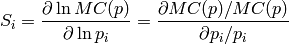
 or
or
 . To work around this, we use a slighly modified
definition:
. To work around this, we use a slighly modified
definition: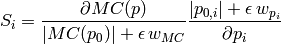
 is assumed to be a typical set of parameter values
(set by
is assumed to be a typical set of parameter values
(set by  terms are
introduced to work around the borderline cases
terms are
introduced to work around the borderline cases  .
.
 corresponds to 80% of the original sampling range and
 is constructed from this.