Professor tutorial¶Contents Creating parameterisations¶Overview¶In this exercise you will learn how to inspect an already produced Monte Carlo dataset with Professor. Please download the dataset (produced with Rivet) from HepForge (lep-exercise.tar.gz) and extract the archive with tar xzf lep-exercise.tar.gz. You will find a directory called mc with 50 sub-directories. Those represent the individual generator runs. The generator output is stored in files called out.aida, the corresponding parameter values can always be found in a file called used_params. The other directory, ref, contains reference data that you try to tune to later. The sample was created using the fragmentation parameters in file trunk/fpythia.params with the tool prof-sampleparams. Envelope plots¶The first step is to look at the individual Monte Carlo runs. The quickest way to get an overview on how well the generator runs “enclose” the experimental data is to produce envelope plots (hence the name). This is done fairly simple: cd lep-exercise
prof-envelopes --datadir . --weights weights --outdir envelopes
This creates a .dat file for every observable that is listed in the weights file weights (see Weights file syntax) in the subdirectory ./envelopes/. prof-lsobs can be used to conveniently make your own weights files in future. You can now use make-plots to produce PDF files: cd envelopes
make-plots --pdf *.dat
The outcome should look similar to this plot: 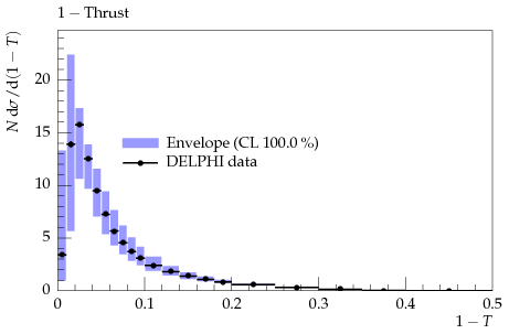
Optionally, if you have installed Professor by yourself or have access to the CERN AFS space to create a simple HTML gallery of these plots you can use the makegallery.py script that is distributed with the Professor source in the contrib/ directory. Type PathToProfessorSource/contrib/makegallery.py (or ~jvonsegg/build/professor-current/contrib/makegallery.py for CERN AFS) in the envelopes/ directory. Parameterising the generator response¶First of all you need to select the MC runs that should serve as anchor points for the parameterisation. The choice of MC runs is stored in run combination files, simple text files, that contain one choice of MC runs on each line. In this example we choose to select all available MC runs only. The run combination files are created with prof-runcombs. To create the run combination file for this example, use in the lep-exercise/ directory: prof-runcombs --mcdir mc -c 0:1 -o runcombs.dat
This creates a file runcombs.dat that contains only one single line with all the available runs. Note To be sure that the parameterisation is not biased by the specific choice and location of the anchor points, it is common use to select more than one set of MC runs, let’s say 100. See prof-runcombs for more information about how to do this. You can now use this file to parameterise the generator response. All you need to do is to run prof-interpolate as such: prof-interpolate --datadir . --weights weights --runs runcombs.dat --ipol quadratic
This will create a single file that contains the parameterisation of the generators response for all bins in all the observables in the file weights. The interpolation is stored in the directory ipols/. We actually made you do a little more work that was strictly necessary for this task: if you omit the –weights and –runs options to prof-interpolate, then all observables in all available runs will be used (each observable with weight=1). But you will definitely want to use restricted run numbers, and put different weights on different observables, so it’s no bad thing to see how right from the beginning! Note Depending on your compiler, prof-interpolate may print warnings, when run for the first time. The reason is that Professor uses on-demand C-code compilation to speed-up the interpolation computations. This is done only once and then cached e.g. in $HOME/.python25_compiled/. Observable selection¶Now it is time to find out which observables are sensitive to the parameters we are going to tune. Interactive exploration¶If you have matplotlib and wxPython installed on your machine, you can use the interactive explorer prof-I. It is called as such: prof-I --datadir ./ --runs runcombs.dat --ipol quadratic
There are a lot more options, so please refer to the instructions found in the documentation for prof-I. Sensitivity plots¶It is also possible to make 2D or 3D sensitivity plots. This allows for a quick overview of the sensitivity of all the observables to shifts in parameter space: prof-sensitivities --datadir . --runs runcombs.dat --weights weights --plotmode extremal -o sensitivity_plots --ipol quadratic
prof-sensitivities --datadir . --runs runcombs.dat --weights weights --plotmode colormap -o sensitivity_plots --ipol quadratic
This creates sensitivity plots in the directory sensitivity_plots/. Tuning to reference data¶Overview¶In this tutorial you will learn how to use the tuning stage of Professor. It is your task to find out which parameter settings were used for the production of the reference data. That’s right, you are not tuning to real experimental data but a MC generator run just like the others in the mc sub-directory. The challenge is to pick observables sensitive to the five parameters that were varied and to tune to this dataset. If you were successful with the first part you should have a folder ipols that contains a generator parameterisation file and a runcombinations file runcombs.dat. Professor tuning¶The tuning stage is accessed using the following command: prof-tune --datadir . --runs runcombs.dat --weights weights --ipol quadratic
This will produce a ResultList with only one MinimizationResult, stored in the folder tunes. Furthermore a file histos-0.aida that contains the prediction of the histograms coming from the generator response will be stored in the folder ipolhistos. You can plot the histograms using some tools of the Rivet package: rivet-mkhtml tunes/params-tune*/*.aida
This produces a web page that can be accessed via the file plots/index.html. Alternativly you can use: compare-histos -R tunes/params-tune*/*.aida
make-plots --pdf *.dat
and makegallery.py from the Professor source distribution to create a simple HTML table, as mentioned above. You can investigate the minimisation-results any time using the command: prof-showminresults tunes/results.pkl
In order to have a look at the histograms, as predicted for any other parameter point you can create a file similar to one of the used_params files in the mc/XXX directories. Let’s call this file prof.params and choose parameter values somewhere within the sampling ranges: PARJ(21) 0.5
PARJ(41) 0.5
PARJ(42) 1.3
PARJ(81) 0.35
PARJ(82) 1.8
To create a file with the predictions of the parameterisation for the histograms in runcombs.dat use: prof-ipolhistos --datadir . --weights weights --runs runcombs.dat --pf prof.params -o myhistos
You can of course also use prof-I for that. E.g. within prof-I hit CTRL+L and navigate to your AIDA-file of choice. Or you can hit CTRL+P, navigate to your prof.params file and click “Set params” to adjust the sliders accordingly. Visualise result scatter¶If more than one run combination was used for tuning to check that the result is not biased by the specific choice of MC runs, the scatter of the minimisation results for these different sets of runs can be visualised with prof-plotresultscatter: prof-plotresultscatter tunes/results.pkl
This produces one plot for each parameter included in the tune in the directory ./resultscatter/. The respective parameter values are plotted along the x-axis, the goodness-of-fit value along the y-axis as in this plot: 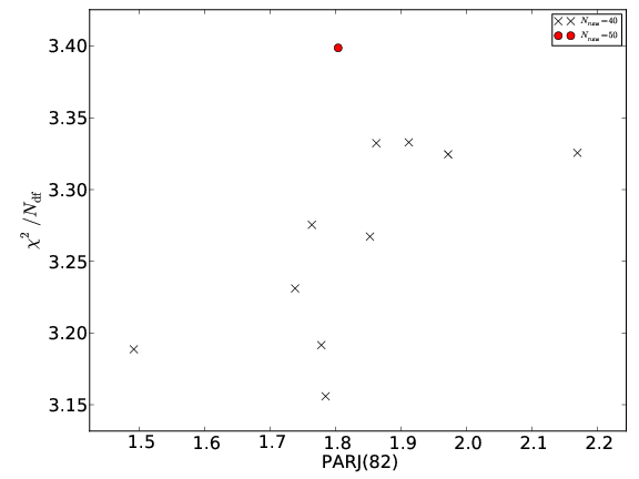
|